Predicting Future Conditions

How does Horizons predict asset deterioration?

When running a Treatment Set or Works Plan, Horizons begins by resampling the surveyed condition data into fixed-length subsections (determined by the Treatment Set). This improves data processing efficiency and makes it possible for Horizons to analyse different survey types with varying resolutions.

Horizons can then predict the future condition of each subsection (if left untreated) by extrapolating from historic data or applying a user-defined curve.

For each Condition Parameter, the last known value is obtained from the most recent survey data available for the subsection. Horizons then calculates a deterioration curve for the parameter, based on the trend of all its historical values on that subsection. Alternatively, you can define a non-historical deterioration curve. This can be linear, quadratic, based on useful life, or fully customised with each point of the curve defined manually.

Per Asset Group

Each Condition Parameter has a separate deterioration curve for each of your Asset Groups.

This is because assets are typically grouped by characteristics such as material type, XSP, construction type or traffic load, e.g. A-roads or B-roads, Urban or Rural, Asphalt or Concrete. Different materials have different resistances to wear and weathering. Assets used more often will degrade quicker. Therefore, the rate of deterioration and subsequent timing of maintenance is expected to be different across these Asset Groups.

They are combined to calculate a mean deterioration curve for each Condition Parameter, which simply describes the changing value of condition over time.

Calculating a deterioration curve

Future condition can be calculated directly from a historical (or other) deterioration curve for any given Condition Parameter. Using a deterioration curve for forward prediction allows the future condition of each subsection to be individually projected, based on its last known condition value.

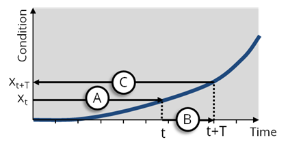
In the following diagram:

• x_t is the current condition
• t is the time the subsection has taken to get to this condition (i.e. to now)
• T is a time in the future
• x_t+T is the condition at this future time

Step A is to locate the current condition (x_t) on the curve, which also identifies the time taken to reach that condition (t).

Step B is to calculate the time (T) in the future by moving the required amount along the time line beyond time t.

Step C calculates the corresponding future condition (x_t+T) by referring to the condition value at time T.

So, by projecting along the curve, the likely future condition can be determined.

Visualise predicted conditions

It's possible to visualise predicted future values of Condition Parameters across your Network assets in the Explorer module. Using specially generated Layers, you can display colour-coded overlays on the map, and select a Section to plot its predicted values in the Graphing panel.

To arrange this, please contact Causeway Support.

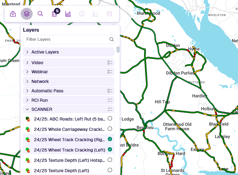
On the map

To view predicted Condition Parameter data on the map, select the relevant Layer (if available):

1. In the Explorer module, click the top Layers icon.

2. In the dropdown, open the folder for the corresponding survey type (e.g. SCANNER) and then select the desired Condition Parameter Layer for the year of interest.

To learn more, see Viewing Data.

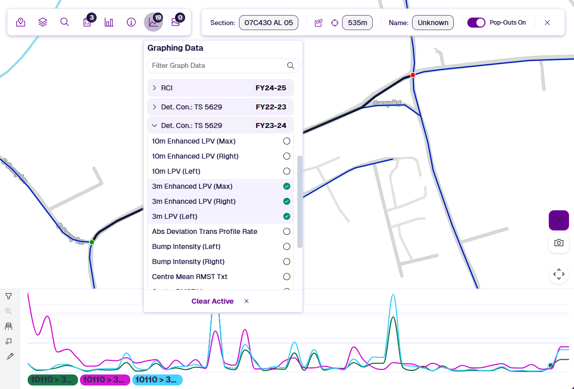
In the Graphing panel

To view predicted Condition Parameter data in the Graphing panel (if available):

1. In the Explorer module, select the Section you want to examine.

2. Click the top Graphing icon.

3. In the dropdown, open the folder for the deteriorated data of interest, and select the desired Condition Parameter.

To learn more, see Understanding Graphs.